

Spectra and Time Loops
We're going to begin this one with a science fiction story. On the way to the international space station, your capsule is intercepted by a ship that seems to suddenly pop into existence—violating at least the speed of light, if not other physical limits you thought you knew about. You are removed from your capsule and locked inside a room with only one window looking out to a corridor. Every day you see a pair of robots approach each other in the same way, then “speak” to each other with the same series of noises, then leave the corridor in the same way. While at first you think these robots are just following some strictly programmed routine, after a while paranoia sets in, and thinking about the impossible appearance of the ship, you wonder whether these alien entities might have some control over time, too. Maybe your cell is stored in some kind of time loop, and the robot interaction that you're witnessing isn't just a repeated interaction, but is in fact the same interaction. Maybe you can find the splice point, you think, the point where time is looped. In fact, the lights do suddenly turn off at one point in time, and gradually come on at another point. Is that the splice point? But maybe the lights are just programmed to shut of at one exact point in time. Maybe, if there's a time loop at all, it's not at that point in time. Maybe everything is lined up exactly and time is spliced during the gradual increase in the lighting. Or maybe there's not a time loop at all. You tell yourself not to be paranoid. But the problem is, without more information, you don't really have any way to tell the difference between repeated events and looped time.
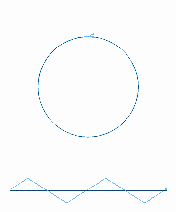
While you may have some legitimate experiential and philosophical objections to confusing the two, analytically speaking there is no distinction between perfectly repeated events and looped time. A periodic wave always does the same thing during each period. Because of this, we can either view a periodic wave as a series of events which repeat in a period \(T\) seconds long, or as a repeating loop that is \(T\) seconds long. As a practical example, If you record 20 cycles or 100 cycles of a perfectly periodic signal into a sampler, the effect is the same. The sampler loops its sample anyway, so it will output the same thing. Of course, analog oscillators and real world sounds aren't actually perfectly periodic, and there might be big differences in practice.
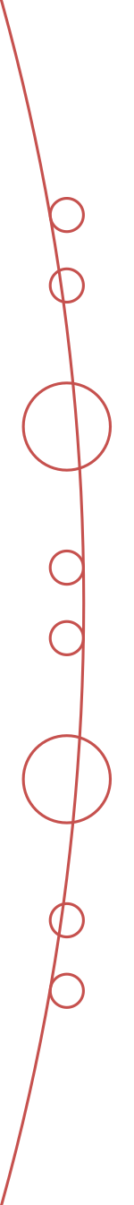
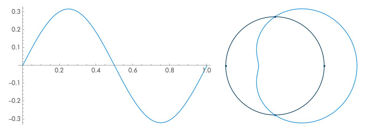
When we represent a periodic wave with period \(T\) in a time loop of length \(T\), we can represent the infinite length of that wave with only one cycle. To move forward in time, we move clockwise, and counterclockwise to move backward in time. We never run out of circle, so all times are represented. Because the wave repeats each cycle, it forms a closed shape on the circular axis, and each subsequent cycle just traces the shape of the previous cycle. With a circular timeline, there is no real beginning or end. But if we fix the rotation of this circle, if we arbitrarily decide that one point in the time loop is going to be on the top of the circle, then the relative phase of the wave in this loop just determines the orientation of the shape. The amplitude, on the other hand, just determines the size of the shape, and doesn't affect its orientation. Note that when the amplitude is large enough to pass through the center of the circle, a twist is created. There is nothing special about these twists. They just come about since anything past the center of the circle is on the other side of the axis of rotation.
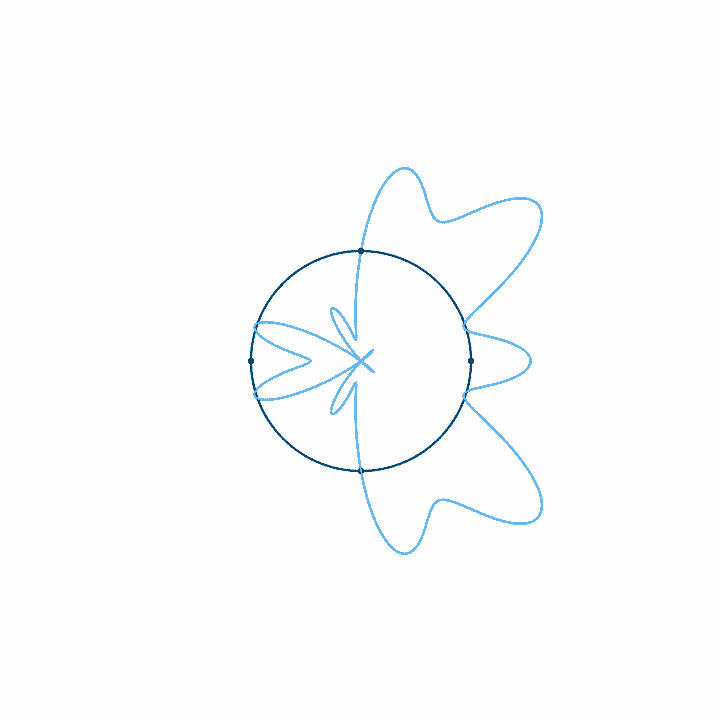
Looping time in this way is not just a method of representation. It's also a way to analyze the relationship of any arbitrary signal to any arbitrary frequency. That is, looking at what a wave looks like with time looped at length \(T\) tells us how that wave relates to the frequency \(f = 1/T\). If, for example, we plot the wave with time looped at some integer multiple of the period of the wave, \(n T\), we get a completely balanced, symmetrical shape—which should make sense, as we must be repeating the wave exactly \(n\) times before we loop. If we loop some unrelated time period, on the other hand, the period of the wave doesn't line up with the duration of the looped time, and so with each loop the wave covers more area, until eventually all areas are evenly covered. Last, if we plot the wave with time looped at some integer fraction of the period \(T / n\), the wave will loop around \(n\) times before it repeats.
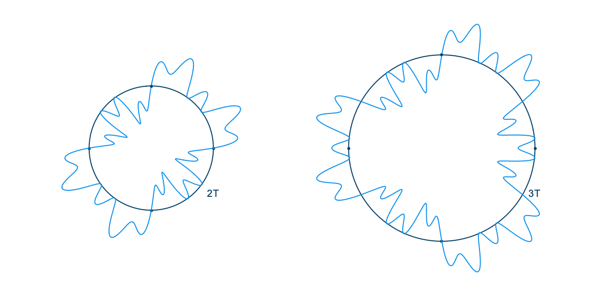
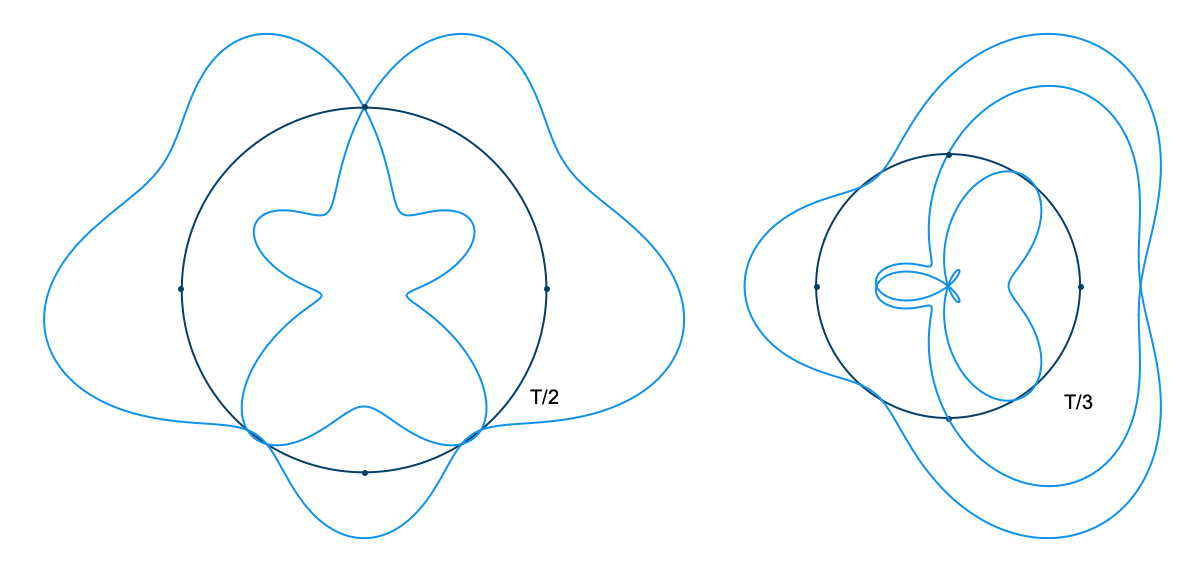
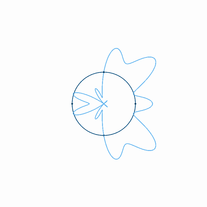
In one sense, a periodic wave has only one frequency, which is determined by its period. But in another sense, a periodic wave seems to be related to a lot of different frequencies. What is the nature of these relationships? Intuitively, we might say that a wave corresponds to a frequency, or that it has content at a frequency, if during the time period for that frequency, the amplitude consistently first increases and then decreases, or first decreases and then increases. This is just a more exact way of saying that there is some sort of oscillation, some sort of back and forth, at that frequency. Consider the case where a wave with the period \(T\) also has frequency content at \(T/2\). With time looped at \(T/2\), the wave will wrap around twice, and because the wave is oscillating, because it is moving back and forth at a rate of \(T/2\), the two wraps will correspond with each other, each one reinforcing the motion of the last. If, in contrast, there was no frequency content at \(T/2\), the two wraps would cancel each other. That is, whatever happened during the first half of the wave won't be correlated with what's happening during the second half. There won't be any consistent motion back and forth at that frequency.
When we plot waves in time loops where they do have frequency content, that motion back and forth translates to motion above and below the axis of the loop, outside and inside the circle. Because some kind of back and forth happens at the frequency we're examining, the plot will have an overall direction. During one part of the loop the wave will be outside the circle, during another part it will be inside, and multiple wraps around the circle will more or less line up. The size of this overall direction will depend on the strength of the correlation and the amplitude of the signal.
Spectra and Sine Waves
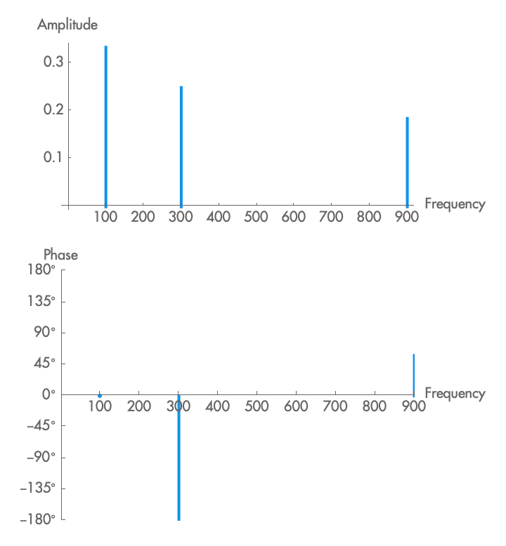
Mathematically, we can get exact numbers for the direction and the strength of this overall direction, and these numbers correspond to the phase and amplitude at that frequency. This transforms a wave from the time domain, in which we know the amplitude for a particular time, to the frequency domain, in which we know the amplitude and phase for a given frequency. The representation of a signal in the frequency domain is also known as the spectrum of that signal (plural, spectra). A spectrum tells us how strongly a signal correlates with itself when time is looped at a particular frequency, and it tells us the phase of that correspondence relative to the time loop. There are multiple ways to visualize a spectrum, but the most common is with two separate plots: amplitude as a function of frequency, and phase as a function of frequency. Often the second plot is omitted, only showing amplitude as a function of frequency.
For perfectly periodic signals, the spectrum will be zero at all frequencies except \(f, 2 f, 3 f...n f\), as at any other frequency the wave either creates a symmetrical shape (for \(f / 2, f / 3...f / n\)), or wraps around continually. But now that we have a method to produce a spectrum, we can use it on signals that are imperfectly periodic. As you would expect, with such signals some frequency component might drift a little between values, or fade in and out, and this will produce a spectrum with a frequency correspondence over a range of values. We can even produce the spectrum of nonperiodic signals, such as noise. A white noise signal, for example, will have frequency components evenly and randomly distributed across the whole frequency range. When a signal has zero content for most frequencies, each frequency (or narrow frequency range) in which it has content is known as a partial of that signal, and the partials are numbered beginning with the lowest frequency, as the first partial, the second partial, etc.
In addition to transforming a signal into its spectrum, we can go the other way, and transform a spectrum into the signal that produced it. A spectrum is unique. That is, given a spectrum, only one signal could have produced it. Suppose that there was a particular wave shape that had frequency content only at exactly one frequency, and zero frequency content at all other frequencies. Because a spectrum is unique, when we add together waves taking this shape at frequencies, amplitudes, and phases according to the spectrum of the original signal, we will have produced the spectrum, and so we will have also produced the original signal.
There is in fact such a special wave: a sine wave. Because a sine wave corresponds with only one time loop, we can take a spectrum and add together sine waves, adjusted according to the frequency, amplitude, and phase of each element of the spectrum, and get back the original signal.
In synthesis, instead of starting with a signal, we often start with an idea of a spectrum we would like to produce. By adding together sine waves at particular frequencies, amplitudes, and phases, we can produce a signal with an exact spectrum. This is known as additive synthesis. While this process is very flexible, that flexibility necessarily comes with complexity—each frequency in the signal has to be specified and controlled. With very bright or very noisy waves, this could mean thousands of frequency components. Because of this, while there are many ways to use additive synthesis effectively, it is overall best suited to signals with only a couple dominant frequency components.
Interpreting Spectra
A spectrum is something we produce by analyzing a wave according to the concept of frequency. But what exactly does a spectrum tell us about a wave?
From one point of view, because any periodic wave can be reconstructed by adding scaled and shifted sine waves, we can think of a wave as already being “made up” of a series of sine waves. Then, analyzing the spectrum of a signal would be like separating the signal into its component parts, or like discovering the chemical formula that tells us which atoms make up a given molecule. The problem with this point of view, however, is that if all we wanted to do was to decompose a wave into a series of scaled and shifted waves of a single type, these waves don't have to be sine waves. Actually, we can use any kind of wave whatsoever. (Consider that for any two waves, there will be a way to scale and shift one of these waves so that when we subtract it from the other, we end up with a smaller wave. We can do that again with the smaller wave: scaling, shifting, and subtracting the second wave and getting an even smaller wave. We can repeat this until the residual wave is arbitrarily small.) This being the case, why not say that waves are “really” made up of a series of some other kind of wave, like square waves?
Another way to think about spectra is as the mathematical analog to what our ears do. Before generating any nerve impulses, our ears separate a sound into different frequencies, and push these different frequencies toward different sensory cells. This has limitations, obviously, as ears are not mathematically perfect, but the way our ears analyze frequency produces results very similar to a spectrum. When we dig further, however, we will find differences. For example, we map sounds out in time in a way that is not entirely like a spectrum. Also, we tend to perceptually ignore some frequency content (among other things, this makes efficient MP3 compression possible). And lastly, while we are still working to understand how we perceive the relative phase of the elements of a spectrum, it is at least clear that we are not immediately conscious of the individual phase relationships between each frequency we're hearing.
Last, although I will address this more fully in a later post, in the physical world, where sounds don't last forever, we can't analyze a spectrum without some amount of uncertainty. That is, while we might be able to deconstruct a wave into a set of sine waves by analyzing it during a certain period of time, we don't know for sure what the wave was doing before that time, and we don't know for sure what it will do after that time. This is true even if the wave is perfectly periodic, since there might be some frequency components that only produce effects in a time frame longer than the one we analyzed. This fact is compounded by the way we experience waves in time. They don't exist forever, and so we would like to be able to say both when a sound started, and when it changed, and what its frequency content is at those times. But these goals conflict: the shorter the time for which we analyze a spectrum, the more uncertain we are as to what its frequencies are; and the longer the time, the more uncertain we are as to when its frequency content changed.
We should be especially wary of interpreting the lower frequencies of spectra where our idea of time conflicts the most strongly with our idea of frequency. At 160 bpm, a pattern of eighth notes will happen at 5Hz, sixteenth notes at 11Hz, and thirty-second notes at 21Hz. This means that, depending on the shape of the signal, we can hear a signal at 21Hz as either a series of really fast notes or as a single note. A spectrum doesn't have the ability to interpret things contextually, and will always just tell us that there is some frequency content at 21Hz.
The spectrum abstraction tells us a great deal about the relationship between a wave and various frequencies. But it does not tell us everything. And there are other ways to think about these relationships. The relationship between a wave and a time loop shows us the complex way in which a wave exists at a given frequency. There are elements of this interaction which are less clear when we reduce the time loop to a single amplitude and phase. Even so, often what we actually care about is not the interaction between a wave and a time loop, but between two different waves at different frequencies and phases, or between three or more waves. The spectrum is an extremely powerful tool of analysis, but because it is so powerful, we have to be all the more cautious not to look for an answer in this bright light, when our question points us to the dark.
Representing Spectra Mathematically
Most often, spectra are represented graphically, as described above. However, sometimes the elements of a spectrum will follow a particular pattern, and so it becomes more useful to represent this mathematically. Generally we would represent a spectrum as the sum of sine waves, using sigma notation.
Sigma notation is just a shorthand way of writing the sum of many terms. The above expression is the same as:
We would read this as: a spectrum (or a sum of sine waves) of the frequencies \(f(n)\), where each frequency \(f(n)\) has the phase \(\phi(n)\) and the amplitude \(A(n)\). Here, \(f(n)\), \(\phi(n)\), and \(A(n)\) are arbitrary functions that specify, for each term from \(n=1\) onward, what frequency, phase, and amplitude the spectrum has for that element. This looks complicated, but in practice these functions can be replaced with simple expressions. For example, this is the formula for a sawtooth wave:
Here we have a spectrum with only a single phase (\(\phi(n)\) is always zero). It has waves with the frequencies \(2 \pi n f\), or all the positive integer multiples of \(f\). The \(2 \pi\) is there since we normalize the sine function such that one period is \(2 \pi\), rather than \(1\). We could instead use the symbol \(\omega\), a lower case Greek omega, which conventionally means the same as \(2 \pi f\). The amplitude of each of these frequencies is \(1/n\), so the first one is \(1/1 = 1\), the second is \(1/2\), the third \(1/3\), etc.
Calculating Spectra: The Fourier Transform
This section will present the actual mathematics for calculating the spectra of a given wave. It requires an understanding of single variable calculus, and ideally, an understanding of complex numbers. There's not much here that isn't already in the intuitive description above, so feel free to skip over this section if you don't want to do this math.
Starting with the description of time loops above, we want to make two modifications. Stretching a period of time into a circle gives us a nice idea about how waves interact, but as things get closer to the center of the circle, they get squished closer together, with the result that positive motion seems to have more of an effect than negative motion. What's worse, this scaling is arbitrary, since it's determined by the relative scale between the units of time and amplitude, and these units aren't really comparable.
We can solve both of these problems by shrinking the size of the circle until it is a single point in the center of the graph, but keeping the length of the time loop the same. Now negative and positive motion are scaled in the same way, and correlations become more obvious. All we really need, then, is to rotate the signal around the axis at a rate of rotation equal to the frequency in question.
Once we have that, we get the weighted area that is inside the graph—that is, the area of the graph, taking the positive and negative directions into account on both axes. This gives us a magnitude and a direction, which are the amplitude and phase of the sine wave at that frequency. To take the weighted area, we take the two-dimensional integral of the graph for the entire wave.
The easiest way to do this mathematically is to use complex numbers. In particular, we use Euler's formula, which tells us that \(\operatorname{e}^{i \theta} = \cos(\theta) + i \sin(\theta)\). Multiplying by an amplitude gives you that amplitude rotated around the origin by the angle \(\theta\). You don't really need to understand the formula however. If we didn't have it, we could just use some other way to wind the wave around the origin at the rate of the frequency in question. Once we have wound it, we take the integral over the entire wave, from the beginning of time to infinity.
Putting this all together, we get the following equation:
This relationship transforms a function of time (\(\operatorname{wave}(t)\)) into a function of frequency (\(\operatorname{spectrum}(f)\)). This function produces a complex vector, indicating the rotation (phase), and amplitude of the signal at that frequency.
There are specific algorithms that are used to calculate the above integral very quickly on digital computers: the fast Fourier transform, or FFT. I won't usually get into particular algorithms in this series, as any algorithm to calculate something should match up with any other method of calculation, and fast algorithms aren't usually the best way to explain a process. It's good to know, however, that this transformation is relatively efficient, and that we can write digital code that relies on it without becoming too slow.
References
For a similar explanation of spectra, see “But What Is the Fourier Transform?” by Grant Sanderson from 3Blue1Brown.
For an introduction to Euler's formula, see “What is Euler's Formula Actually Saying?” by Grant Sanderson from 3Blue1Brown.
For more on the Fast Fourier Transform, see “Fast Fourier Transform (FFT) Algorithms,” In Mathematics of the Discrete Fourier Transform, by Julius O. Smith.