


On Audio Fidelity: Measurement
Part 2 of 3
In 2011, an experiment at CERN measuring the speed of neutrinos seemed to show that they were travelling faster than light, which, if true, would probably violate the principles of special relativity and in turn undermine a lot of modern science. The vast majority of the scientific community was immediately convinced that this was anomalous, that the results were due to error, not observation. But scientific error must also be explicable, and so there was a flurry of examination and theorization about the way their measuring devices worked, in order to locate this error. Fortunately for relativity, the error was successfully modeled, which means that the models of the measuring devices were changed, and consequently the measurement itself was retrospectively altered.
Measurements always depend on the models that create them. Conversely, measurements provide the evidence for a model’s accuracy and correctness. This does not mean that models aren’t built on evidence—this is just what scientific evidence is. If it seems like the only thing you could possibly prove with such a system is whether the whole thing is coherent or self-contradictory, welcome to modern science. It is the source of awesome power and nuanced comprehension, but unassailable truth is not part of its remit. If you want more than coherence (and everybody wants more), you will need religion, philosophy, or art.
In the fidelity model, a series of measurements are used to quantify the differences between the audio a system produces and the audio it “should have” produced based on the recording. From the other direction, the fidelity model uses these same measurements to determine the difference between what an audio system records and what it “should have” recorded from a sound traveling in the air (or from another recording). So long as these two measurements indicate no differences, the correct sound will supposedly be produced.
The contents that a recording “should contain” could be defined as whatever would make the sounds perfectly correspond when both the recording and playback measurements were perfect. However, without some prior definition of how the correspondence between recording and measurements should work (without some model), there would be no way to determine whether the deviation was in the recording or in the equipment. There are actually several different ways to model this correspondence, and we will look at them in part 3. But they all begin by simplifying a sound to a set of one-dimensional signals (see Approaches to Sound), one signal for each channel, where the signal amplitude corresponds to sound pressure in the air. The deviation of the recording and playback systems can then theoretically be characterized according to this abstract definition of a recording, and each element of the system can be tested separately—the electronic elements according to the correspondence between input and output signals, and the transducers (microphones, speakers, pickups, etc.) according to the correspondence between signal level and sound pressure level (SPL). However, in adapting this model to modern studio recording techniques, this signal is reimagined as something that originates with the intentions of the composer, mix engineer, etc.
While there are a few more obscure measurements that are occasionally provided, generally speaking fidelity is measured with frequency response, phase response, total harmonic distortion, and noise level / dynamic range. We can break all these measurements into three broad categories: frequency and phase response (linear differences), distortion (nonlinear differences), and noise (uncorrelated differences). I’ll address these in that order, and give an overall conclusion at the end. This post is long, so feel free to bookmark it and skip around.
Measurement: Frequency and Phase Response
The frequency response of a system is a comparison, in decibels, of the spectrum of an input signal and the spectrum of the signal after passing through the system. Each frequency is given a measurement according to its deviation, but often the entire frequency response is characterized by the maximum deviation over a frequency range, for example 20Hz-20kHz ±1dB. Note: in reading a frequency response graph, or any exponential graph, always refer to the labeled scale. Any exponential graph can be made arbitrarily close to a straight line by choosing the appropriate scale, and for marketing reasons manufacturers often choose the flattest scale at which their graph is still readable.
The most intuitive way to measure frequency response is with a sine wave that gradually increases from low to high frequency, known as a sweep tone or chirp tone. The amplitude at each frequency is measured and compared with the average amplitude, and the resulting graph is the frequency response. At the same time, the input phase can be compared with the output phase to obtain the phase response. The disadvantage of this method is that it doesn’t provide instantaneous feedback. Alternately, frequency response can be measured with a noise signal. Since noise contains all frequencies, you can compare the spectrum of a noise signal at the input and the output in order to determine the phase and frequency response. Actually, any known signal can be used, including music, although of course the frequency response can only be measured for frequencies that are present in the input signal’s spectrum. When humans are very familiar with how a sound “should” sound, such as white noise, we can use it to estimate the frequency response by ear. However, we are only sort of okay at it. Our ability to mentally recall and compare sound is much worse than our ability to hear in the first place.
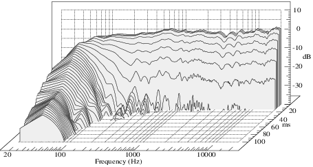
While it’s less common, the relationship between the frequency response and the temporal response can be measured with a three-dimensional waterfall plot. A waterfall plot indicates the way that a system stimulated at all frequencies gradually decays over time. Waterfall plots help visualize how resonances in the frequency response will affect the timing of a sound. In the ideal case, the waterfall plot would have a straight line in back, representing a perfect frequency response, and nothing in the rest of the graph, representing an immediate decay into silence when the sound is removed. Practically, all systems will have some decay, but briefer decays, more spread out through the frequency response, will be better. A waterfall plot is either made by measuring the decay individually for a set of frequencies and interpolating between them, or by first creating an impulse response (the response of the system to a sudden click), and then analyzing that impulse response as an evolving spectrum. These can give slightly different results.
In signal-level electronics—anything which does not have to drive physical speakers, headphones, or cutting lathes, and which is not driven by microphones, cartridges, tape heads, etc.—a frequency response of better than ±0.1 dB from 1Hz-35kHz is not particularly difficult to achieve, with the most common deviations appearing in the lower frequencies, for devices which block DC (absolute voltage offsets, or 0Hz), and in the upper regions, due to the limited speed of the response of the electronic system itself, as well as from intentionally applied filtering to avoid unwanted high-frequency signals. In power amplifiers, figures like this are considerably more difficult, but still achievable. In digital converters, nearly perfect frequency responses within the audio range are fairly easily achievable.
Note that in preamplifiers that produce a signal from physical vibration, such as a microphone or phono preamp, the input stage interacts with the object producing the signal (the microphone or cartridge) in complex ways. While manufacturers of these devices can and should try to optimize the frequency response in abstraction from this complex interaction, note that our model of measurement deliberately abstracts from these kinds of interactions, and may not adequately predict the complete result.
In speakers and headphones, frequency responses are less accurate. In studio monitors, ±2-3dB from 100Hz-20kHz is achievable—this is, for example, the frequency response of Yamaha NS10s. Generally a speaker will have peaks or valleys in crossover points (one for two drivers, two for three), plateuas when one driver is more sensitive than another, a steep drop off and perhaps a hump on lower frequencies, and some wildness at the top of the range where the wavelength of the sound starts to become comparable to the size of the speaker. In particular, speakers have a lot of difficulty reproducing the bottom of the range, and generally need to be physically large in order to do so. While it is difficult to get measurements for large and expensive mastering or hi-fi speakers, they don’t seem to be able to improve much on the 2-3dB variation. They do, however, extend the range over which this variation is valid down to 20-30Hz and up to 25-35kHz or so. Also, sometimes within a much smaller frequency range, say 250Hz-2kHz, these expensive speakers are able to achieve something less than ±1dB. Even the largest speakers struggle to produce sounds below 20Hz, for which one likely needs a large, dedicated subwoofer.
Headphones are generally much, much worse, with ±12dB from 30Hz-8kHz being fairly common for good headphones, and ±4dB from 20Hz-8kHz nearing the best achievable. Headphones tend to extend lower than small speakers, but not to the bottom of the audio range. At the top end, from 8kHz-20kHz, most headphones exhibit a ton of random variance, as much as ±15-20dB, as their shape as well as their position over the ear creates many resonant modes in the high frequencies. Further, because the sound from a headphone is not affected by the ear in the same way that normal sounds are, a perfectly flat frequency response is generally considered undesirable. If we wanted to exactly reproduce what “would have been” heard on perfect speakers, each headphone would need a frequency response that was exactly tailored to how each individual ear responds to sound in the air. In practice, headphones compromise with a vague curve.
Microphones can be very, very good, with expensive microphones marketed as measuring devices achieving ±0.5dB from 10Hz to 40kHz, although manufacturing inconsistencies will make guaranteed values more like ±1-2dB. However, accuracy, especially at the top of the range, is going to depend on the relative position of the mic and the sound source. While microphones with a flat response are available, most microphones are not actually designed to be overly flat, but rather to have an overall response that is well suited for their area of application.
Lastly, different rooms and different speaker positions are going to have different frequency responses. ±6dB from 15Hz-10kHz is pretty good for a well-treated room. With a purpose-built listening room and a professional acoustician, ±2-3dB is achievable. Rooms usually have problems in the bass frequencies, when the wavelength approaches the length or width of the room. To get a response this good, you need to treat the room with acoustic panels and bass traps. However, unless one also adopts the concept of a single, set listening position, beyond a certain threshold, damping might not be desirable, since wall reflections help to spread sound evenly through the whole room. Further, we seem to be naturally good at mentally separating the objects we hear from the room in which we hear them, provided we are in that room. We do not necessarily need a perfectly flat, unresponsive room.
What all these numbers should make clear is that while certain kinds of electronics are fairly good, the overall frequency balance you are likely to hear, even on the absolute best available room and speakers, will be colored in a way that is easily perceptible. The idea of a complete system that exhibits a perceptually flat frequency response is wishful thinking.
Correcting the Frequency Response
Can we correct for the frequency response with a graphic EQ or with digital signal processing? Is this a simple problem? If frequency was the only thing we cared about, we could absolutely correct for frequency response. However, when time or phase response is taken into account, the situation becomes much trickier. Nevertheless, because frequency response is such a powerful measurement in marketing audio equipment, and because the problems with correction are less widely understood, manufacturers often do correct for bad frequency responses in various ways, while being silent about the tradeoffs this entails.
At some point I’ll write in better detail how filters work—and every system that changes the frequency response is just a filter, whether intentionally constructed or not. For now, just know that the only way to change a frequency response in a system where time moves forward (any physical system) is to delay some of its energy. Consequently, the only way to perfectly remove this change would be to advance that energy, that is, to move backwards in time or to know the future. The only way to know the future is to use a delay. This gives us our first problem: mathematically, there is always a filter that will exactly reverse the effects of another filter, for both frequency and phase. But if we want to build something like this filter in reality, we’ll have to accept a delay. Depending on the frequency response we want to correct, quite a lot of delay might be needed. Just to accurately know what frequencies we have going in, we need a delay at least equal to one period of the wave in question. At 20Hz, that’s 50ms. For actually constructing the desired filter, we may need a lot more. When listening is the only goal, this delay might not be important. In music production, 50ms is a problem.
Our second problem is that vibrational sound is not actually the one-dimensional object with which we model it. A real room is going to have different frequency and phase responses at each three-dimensional point. Even if we limited our corrections to the speaker alone, we still have a three-dimensional object. Mathematically speaking, it is generally not possible to alter a one-dimensional signal in order to produce the correct signal within a three-dimensional space. If it were possible, we could create perfect spatial audio with a single speaker, or specify an infinite number of channels with a single signal.
As such, generally no attempt is made to exactly compensate for frequency, phase, and timing. Nevertheless, there is currently a lot of active research in using DSP to improve the response of a room or speakers. This can get very sophisticated, but usually manufacturers focus mainly on frequency, just creating a filter with an approximately opposite shape.
However, it is not possible to create a filter without changing timing, phase, or both. To understand this intuitively, let’s visualize the relationship between filtering and delaying energy. When filters attenuate certain frequencies, they steal energy from the present and release it in the future, but out of phase. The energy added in the future has to work against the stored energy, and the signal is attenuated. When filters amplify certain frequencies, they release that future energy in phase, such that energy from the past joins with the energy being presently added by the sound, making the amplitude of the system disproportionately large compared with the energy being added. Because this energy is released in phase, the energy that is released is also partly stored, and released in phase and partly stored, etc. This is resonance, and in resonant filters, it can take many cycles for the energy applied within a single cycle to dissipate.
As a consequence, whenever a filter acts on a frequency, it delays that frequency, at least by one half cycle (to attenuate) or one whole cycle (to amplify), and in resonance, a filter spreads transients out to cover more time. The frequency response that we are trying to compensate for already delays and spreads out the sound. Anything we do to compensate will add further delay and spreading.
Because the same phase differences correspond to longer delays at lower frequencies, these timing distortions are often the worst at the lower end. Unfortunately, this is also usually the weak point for a pair of speakers, especially smaller speakers. Because the frequency response measurement is such a powerful piece of marketing for a speaker, almost all speakers currently made are ported. That is, a hole on the speaker cabinet provides a boost in amplitude over a wide range of frequencies by providing a modest resonance. In cheap speakers, this resonance may be somewhat less than modest, providing completely smeared and boomy bass. A very well designed port will have sufficient damping to prevent a noticable resonance. But the entire point of adding a port is to extend the frequency range of a speaker through boosting lower frequencies, and this is only possible when the resonance is sufficiently high to extend the temporal response at least a small amount beyond the signal.
Our systems aren’t perfect, and which type of imperfection is best will vary depending on the situation and the objective. Correction might be the best choice. But timing, phase, and frequency are inextricably related, and no amount of technological advancement will break that relationship. We can only choose. Unfortunately, with the prevalence of frequency response as a simplified measure for the quality of the system as a whole, all too often the choice has already been made for us.
Measurement: Total Harmonic Distortion
Distortion is any unwanted sounds that a device creates which are related to (or correlated with) the input signal. Sometimes this is also called nonlinearity, or total harmonic distortion, THD. If a device does nothing but amplify a signal, then, other than noise, there will never be frequencies in the output which were not present in the input. The map from input to output, in this case, looks like a straight line. If anything nonlinear happens—if the map is not a straight line—then other harmonics not present in the input spectrum are produced. Distortion is a measure of how straight the line is, based on the spectrum that is produced. To put it another way, distortion is a measurement of how much the amplifiers inside a device just act like amplifiers, without producing harmonics. It is given as the amplitude of all the new freqencies taken as a percentage of the frequencies that were supposed to be there.
Distortion is usually measured with a 1kHz sine wave as input. The amplitude of each harmonic at 2kHz, 3kHz, 4kHz, etc. is measured. This is given as a percentage of the amplitude of the 1kHz wave, for example, 0.05% THD. Sometimes the noise and the distortion are not differentiated, and are given as THD+N. In this case, the amplitude of everything except the 1kHz wave is taken as the noise plus distortion.
While a decibel measurement would allow for more consistent comparisons with other common measurements, traditionally distortion is given as a percentage. However, this percentage can easily be transformed into a decibel value:
For example, 1% THD is -40dB, 0.1% is -60dB, 0.01% is -80dB, etc.
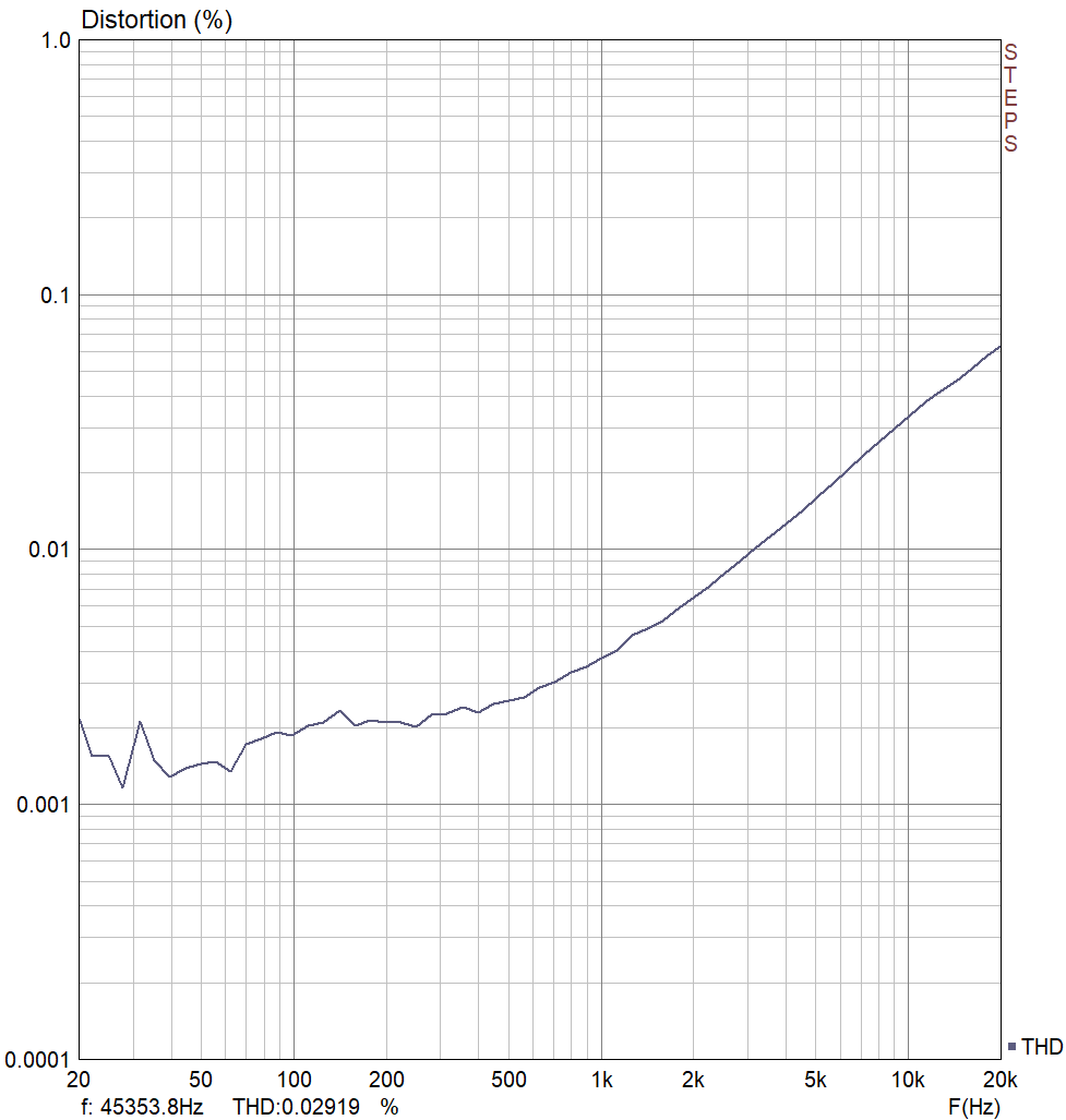
As a measure of nonlinearity, a single value for THD at 1kHz leaves a lot to be desired. First, distortion is always dependent on amplitude, and while some devices will have an amplitude that produces a minimum distortion, others will get arbitrarily better as the signal gets quieter. Second, in most real world devices, distortion is not constant with frequency. Usually, this frequency dependence is not a big deal, but it is just not a universally valid assumption that because there is low (or high) THD for one frequency there will be low (or high) THD for the others. Last, the distortion of a line level amplifier is often dependent on how hard it has to work, which means it could be dependent on the impedance of the following stage. Generally, higher input impedance will lead to lower distortion (but more noise, see below). Because of all these variables, in certain circumstances you’ll see a plot of THD vs. frequency, amplitude, or some other variable.
With simple line level devices (amplifiers that are not voltage controlled), it is fairly easy to achieve a THD of 0.05% (-66dB), with 0.001% (-100dB) fairly typical in a high end device. Theoretically, the best available component amplifier gives around 0.00003% (-130dB) in ideal conditions, but these conditions are unlikely to be met in a complete device. The best DACs can achieve around 0.0001% (-120dB) distortion, with most falling closer to 0.001% (-100dB).
For power amplifiers and preamplifiers, distortion figures of 0.1% (-60dB) are generally achievable, with 0.01% (-80dB) nearing the best possible. However, 1% (-40dB) or worse is not altogether uncommon.
For more complicated devices containing voltage controlled amplifiers or similar (VCAs, compressors, filters, etc.), 1% (-40dB) or worse distortion is relatively common. However, 0.05% (-66dB) is fairly achievable, with 0.01% (-80dB) being around the best currently possible.
Speakers tend to be among the worst devices for distortion, with many high-end and monitoring speakers doing no better than about 1% (-40dB) distortion. Often the worst distortion occurs in the bass frequencies, as much as 5% (-26dB). High end mastering and hi-fi speakers can get more like 0.1-0.5% (-60dB to -46dB). The situation is slightly better for headphones, with typical monitoring headphones being around 0.5% (-46dB) and the best achievable being around 0.05% (-66dB).
Microphones tend to produce distortion that is much worse at higher SPL levels, and so figures for microphone distortion tend to be given as the maximum SPL that can be achieved for a given distortion level, for example 0.5% at 137dBA. Distortion at “normal” levels is not typically published, but it seems like microphones are often quite good, in the 0.01% (-80dB) range.
While the very best line level devices and digital converters will produce distortion that as far as we can tell is not detectable by humans, other electronic devices sit right on the border of audibility, creating distortion that will only be heard in certain circumstances by certain people, if at all. In contrast, speakers commonly produce audible levels of distortion. On the surface, it doesn’t make much sense to worry about other kinds of distortion when speakers are so bad. But unlike noise, quiet but audible distortion will not necessarily be lost in louder distortion, as every distortion curve is a little different and behaves differently with different signals.
Types of Distortion
Distortion is a curve in mapping one amplitude to another. While there is only one straight line that produces a certain amplitude with no distortion, there are an infinite number of different curves that could produce a given THD measurement. These curves sound different and behave differently with different kinds of input signals.
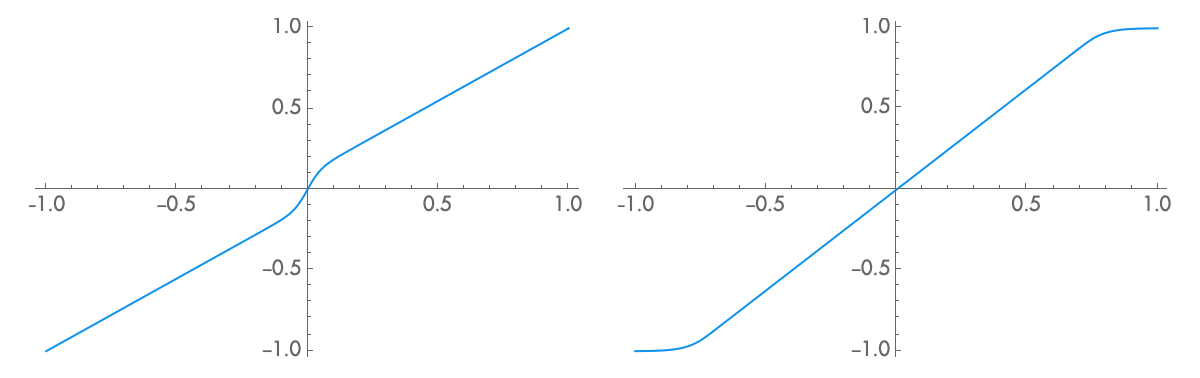
Typical, modern amplifiers produce two kinds of distortion. The first kind, clipping distortion, is more pronounced at the extremes of the waveform, as the device nears its maximum amplitude. The second kind, crossover distortion, happens as the waveform crosses over zero volts. Crossover distortion comes from class AB amplifiers, which divide the signal into positive and negative parts in order to amplify it more efficiently. Inside the device, one amplifier is cutting off and another is turning on, and when this happens there can be a slight glitch which shows up as distortion. Crossover distortion is not typically present in class A amplifiers (including most tube amps).
These two types of distortion sound a little different on a constant signal, but they behave completely differently in response to a dynamic signal. Clipping distortion will be almost completely absent from quieter passages, and gets more extreme with louder volumes. As such, it is at its worst when the output is loud, possibly loud enough to entirely drown it out. Crossover distortion, on the other hand, is typically present in a constant amount, regardless of the amplitude of the input signal. As a consequence, the same amount of crossover noise that is inaudible in a loud passage may suddenly become audible in a quieter passage. Ideally, in order to understand how distortion would work in a particular application, distortion would be measured at both louder and quieter levels. In most modern amplifiers, crossover distortion dominates and distortion is measured at a relatively high output level.
While figures for distortion at other levels are rarely published, crossover distortion often scales linearly as the level decreases. That is, for every -6dB of volume, double the percentage. With a device with a wide dynamic range, such as a power amplifier, this can mean that the actual distortion at a given volume could be seveal orders of magnitude different from the published figures.
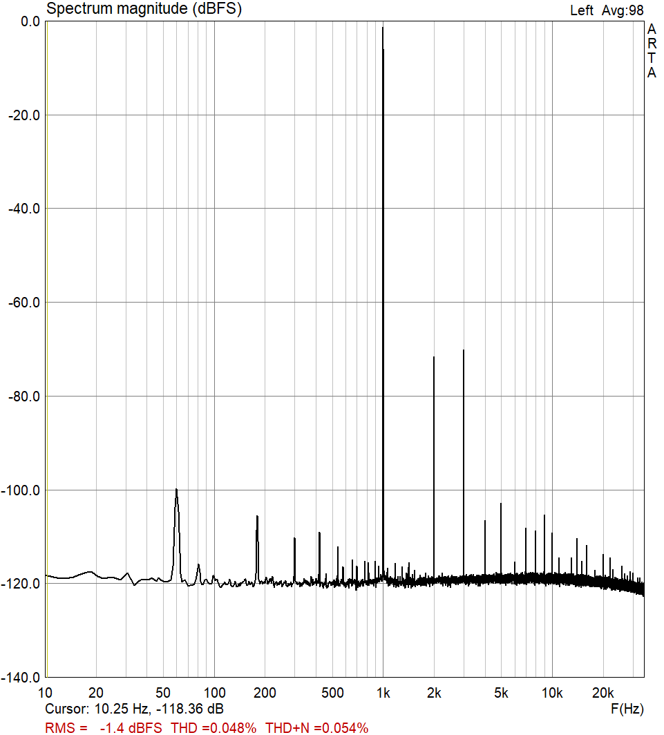
Since the consumer shift to the transistor amplifier and digital electronics in the 70s and 80s, it has become trendy to distinguish between odd and even harmonics in distortion, with even harmonics generally considered to be better. Sometimes this is illustrated with a graph of the spectrum of the output when a 1kHz signal is applied, where the relative value of each harmonic is apparent. Because of the way the mathematics works out, even harmonics are only produced when the map from input to output is asymmetric, that is, when the device does something different for negative and positive amplitudes. Symmetric maps produce only odd harmonics.
This question of symmetry is often mistakenly applied at the level of individual components, with the idea that transistors are symmetric while tubes are asymmetric. In abstraction from a circuit, both devices are heavily asymmetric. The reason for this association actually has more to do with the relative cost of different designs. Manufacturers of transistor amplifiers are incentivized to develop more complicated designs that use more cheap transistors (or integrated circuits) but less power, saving money on big copper transformers. Manufacturers of tube amplifiers are incentivized to use as few expensive tubes as possible, regardless of the rest of the circuit. Symmetric vs. asymmetric is usually just two devices vs. one device within a given amplifier stage, and so transistor designs tend to symmetry, while tube designs tend to asymmetry. When cost is not taken into account, it is trivial to design symmetric tube amplifiers and asymmetric transistor amplifiers. These will still behave slightly differently, to be sure, but the symmetric tube amplifier will have only odd harmonics, while the asymmetric transistor amplifier will have both odd and even. While the question of odd and even harmonics is clearly important for intentionally produced distortion, I would conjecture that crossover vs. clipping distortion is probably the more pressing issue for a clean amplifier.
Measurement: Noise and Dynamic Range
As defined for the purposes of measurement, noise is any unwanted signal that is unrelated to (or uncorrelated with) the input signal. It can be random noise, it can be AM radio, it can be 60Hz or 100kHz hum, etc. However, when noise measurements are considered theoretically or mathematically, generally noise is thought of as broadband noise, that is, a signal spread out over a frequency range rather than consisting of a set of individual frequencies (like pitched sound). Because of this ambiguity, some of the math will not work out exactly correctly when practical noise measurements include discrete frequencies like hum.
The simplest noise measurement is just the average (RMS) amplitude of the total noise in a system. This is usually measured in a limited frequency range, 20Hz–20kHz. Although occasionally noise is measured in absolute units, such as mV or dBA, it is more common to see dB, where the point of comparison for the dB unit is usually the loudest signal level of interest. For this reason, this measurement is sometimes inverted and called the signal-to-noise ratio, or SNR. While noise can be measured just by taking the average output amplitude with no input, often noise and distortion are measured at the same time by recording the output with a 1kHz sine wave input and subsequently subtracting the input and distortion.
Measuring noise in this way gives a pretty good simplification, but there are some edges we should be aware of. First, in something with a volume control, there are usually two kinds of noise: noise which gets louder when the volume is louder, and noise which is constant regardless of the volume control’s position. These systems will often be measured at whatever point the balance of these figures gives the best measurement, and you may find that at lower volume levels more noise is present.
Second, often high frequency hum won’t be accounted for in these figures, as it lies above 20kHz. Many devices have poorly filtered switching power supplies that run around 50-100kHz, and others accidentally produce high frequency signals in other ways. While these signals won’t be directly heard, they may affect other parts of the system. In particular, this has been a problem observed in a few digital converters running at 192kHz and above.
Third, in any electronic device, because the signal is defined in terms of voltage, the noise level will be measured in terms of voltage. But there is always a second noise level, the current noise. This current noise will become voltage noise in different ways depending on the impedance of the following stage. If you find that when connected to some things a certain device is extremely noisy, but at other times it is relatively quiet, current noise might be the culprit. Input impedance in professional audio gear can range from around 10kΩ for a line input to 1-5MΩ for a guitar input. Eurorack, synths, and older gear are somewhere in between at around 100kΩ. This means that the same current noise could result in effective noise levels as much as 50dB apart.
Noise levels for electronic devices range from incredibly good to mediocre. Some synths, guitar pedals, and vintage devices have as bad as -40dB noise levels. The best we can currently get in practical electronics is somewhere around -110dB to -120dB for a line level device. Typical devices used for music production are usually somewhere around -70dB to -80dB, but it is not uncommon to find both better and worse figures. Eurorack modules are often around -60dB, but de facto Eurorack standards keep signals at the louder end of that dynamic range, opting for clipping and reduced dynamics rather than excess noise. While exceptionally careless and exceptionally careful design is possible, often high noise devices are just normal devices with high gain. Starting with the same kind of noise and a quieter signal, the whole thing is amplified and results in a noisier device.
Microphones, phono cartridges, reverb pickups, etc. generally need a lot of amplification, and usually the majority of the noise with these devices comes from the electronics of the preamp. Because this scales with the level of amplification, usually a louder pickup device and a less noisy pickup device are almost the same thing. However, if the device has internal electronics (e.g. FET mics), or if the preamp is very quiet, that may not be the case. While I haven’t seen measurements for other kinds of pickup devices, microphones are often measured for self-noise—the inherent noise of the microphone regardless of the preamp. Most likely, however, this figure does not include current noise, and may shift slightly with the impedance of the preamp.
Noise is not usually an inherent issue for speakers or headphones (they are not randomly pushing air molecules any more than any other object in the room). However, note that the different sensitivity of different speakers will produce different relative volumes for the static part of an amplifier’s noise output (the part that doesn’t change with volume). As a result, more sensitive speakers tend to be “noisier,” even though most of that noise is actually produced by the amplifier. This can be particularly noticeable on headphones, as they are often designed to work with very low power, portable devices.
Despite common misconceptions, software and digital audio is not noise free. For a deeper discussion of this, stay tuned for part 3. For now, be aware that the digital audio medium has an inherent noise floor which is determined by the bit depth. This noise floor is always 1 bit peak to peak, or \(1 / \sqrt{12}\) bits RMS. 16 bits gives an inherent noise floor of -98dBFS (not the often quoted -96dBFS!), while 24 bits has an inherent noise floor of -146dBFS (not -144dbFS!). Note that these theoretical minimums are for undithered noise, which is actually distortion. To replace this distortion with pure noise, generally noise is added at 2 bits peak to peak, or \(1 / \sqrt{6}\) bits RMS, giving -92dBFS and -140dBFS for 16 and 24 bits, respectively.
Noise Floor, Dynamic Range, and Noise Spectral Density
While measuring the total noise level is straightforward, this process is ambiguous in some unintuitive ways. For example, suppose we want to know the noise level in a particular system, so we measure the sound level with a digital audio interface running at 48kHz. Then we go back and do the same measurement at 96kHz. For many devices, the result will be about 40% more noise, a very significant measurement difference, even though in most cases the audible difference between these two recorded sounds would be imperceptible to humans. In fact, as the frequency response of the measuring device and the device being measured grow, the noise level grows without bounds. A theoretically perfect frequency response will always have an infinite total noise level, even if the noise within the audible spectrum hasn’t changed. As I mentioned above, one way to deal with this is to define a frequency range for the measurement, generally 20Hz-20kHz. However, this can obscure less audible issues that might become audible in certain circumstances.
The solution is to measure the noise density at a given point in the spectrum rather than the noise level for the spectrum as a whole. The noise density is related to the RMS noise level from \(f_0\) to \(f_1\) with the equation:
When most of the noise is white noise—broadband noise that is evenly distributed throughout the spectrum—this equation reduces to:
Note that the noise density of a region can only be defined for broadband noise, as a specific pitch would have an average noise density of zero.
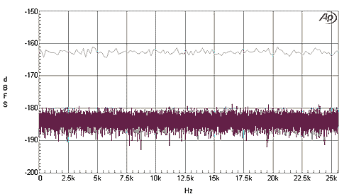
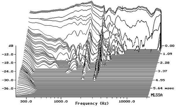
Unfortunately, a lot of measurements unintentionally confuse noise density with the noise level in a small frequency range. A spectrum is produced, and the noisy line on the bottom is read off as if it was the noise density, or the “amount of noise” at that frequency. Sometimes this is erroneously called the noise floor. This has the same measurement problems as overall noise level—the value is entirely dependent on how big the frequency range is, such that a spectrum measured at 20Hz intervals will measure 40% more noise than a spectrum measured at 10Hz intervals. That is, unless you know the precision at which an analyzer is working, the noise level it shows is meaningless. While special purpose noise spectrum analyzers can automatically convert to noise density, correctly analyzing the noise level means incorrectly analyzing the level of pitched sounds, and so no general purpose correction is possible.
The noise floor is defined in various ways. Usually it’s just identical to the noise level, but sometimes other measurements are used. However it is defined, the idea is that there is some level at which sound becomes indistinguishable from noise. These sounds would be the quietest sounds that the system can produce, and the dynamic range would be the ratio of loudest to quietest sound. This theory bears little relationship to reality. From a mathematical perspective, when signal and noise mix together in any amount, there is some small uncertainty as to what the signal is. As the level of the signal decreases below the noise level, that uncertainty increases, but it never becomes absolute. To put it another way, adding a signal of any amount to a random signal makes the resulting signal slightly less than random. Further, one can always decrease the uncertainty by observing the signal over a longer time period. Of course the question of how this affects human hearing is another matter. Certainly, noise masks quieter sounds, but there’s no reason to suspect that this happens abruptly at a frequency-independent threshold.
Noise Reduction
In a recording, noise reduction generally happens through two mechanisms. The first is just expansion, or noise gating: when the material gets quiet enough, the volume of the whole signal is lowered. While this does nothing to lower the background noise while something is actually playing, it makes the silent parts more silent. Because a noise gate is just an expander with a very low threshold, it can create the same kinds of problems (and benefits) as other kinds of microdynamic manipulation. Typically, the issue will be overly abrupt attacks and decays. In particular, decays with a very long tail will often be lost.
The second method can only really be done in a non-real time environment—digital wave editors, such as Audacity or Seqoia, or specialized tools, but not most DAWs. This method typically has two phases. First, some section of audio that only contains noise is analyzed to see what kind of frequencies are in the noise. Second, the audio is processed with what is essentially a multiband expander with hundreds or thousands of frequency bands. The expander is tuned to the frequency profile from the first step, such that noisier frequencies get more agressively gated than quieter frequencies. Because the multiband expander is acting on each frequency independently, it can remove background noise even while other sounds are happening. Note that, since noise is just defined as anything you don’t want, this method can be used to remove literally anything. For example, to isolate the vocals on a track, you can analyze a part of the song without vocals as “noise,” then noise reduce the part with the vocals. This second method is usually implemented with spectral analysis and resynthesis, and it has the same sorts of problems as other effects which use spectral analysis: a tradeoff between temporal resolution and frequency resolution, often leading to strange glitch effects from quantized or overly-sparse frequencies.
A Brief History of Imperfection and Objectivity in Music
Thus was born the concept of sound as a thing in itself, distinct and independent from life, and the result was a fantasy world of music superimposed on the real, an inviolable and sacred world.
—Luigi Russolo, “The Art of Noises,” 1913.
When the fidelity model defines noise as unwanted signal, it transforms aesthetic discussions about the value or beauty of certain kinds of sounds into discussions about the mathematical deviation of a device from a predetermined ideal. In fact, that is the central function of this definition. As soon as one begins to desire some kind of noise, the definition of noise reclassifies this desired noise as signal, and whatever’s left becomes the noise. While this presents a veneer of agnosticism, on closer inspection the only way noise could be a good thing in this model is if it were part of a master plan all along. In defining noise in this way, the model of fidelity is able to present its measurements as if they existed entirely outside of aesthetics, and yet were entirely pertinent to aesthetics.
In contrast, I would conjecture that very few recording artists actually encounter noise in this way. It is not at all unusual for a modern recording to forego noise reduction, or even add some kind of background noise. While there are certainly decisions being made here, people are not generally constructing the entire noise floor as part of the composition process. Instead, this noise is an object encountered within the material process of the production of music, and the decision to leave it in is often a way of foregrounding the materiality and externality involved in the creation of music.
The pursuit of noise in music was one of the central concerns of twentieth century music, and the history of this pursuit is deeply entangled with the larger history of electronic music. This is a topic well beyond the scope of this post. However, two threads of exploration, with a lot of overlap, are especially relevant here.
One focuses on the objectivity of sound, the world of sound, and the way in which this world can be represented in a recording. In contrast to the (unreal) idea of a composer as a masterful wellspring of creativity, music made with this objective approach is often more about encounters, listening, discovery, taste, and reappropriation. Like most important practices, it had multiple entangled origins: the mechanical noisemakers of Luigi Russalo; the musique concrète of Pierre Schaeffer and Pierre Henry; the dub of Lee “Scratch” Perry and King Tubby; left-field studio production practices from Joe Meek and Brian Wilson; the magnetic and optical tape manipulations of Daphne Oram and the BBC Radiophonic Workshop; the turntablism of DJ Kool Herc, Grandmaster Flash, Grand Wizzard Theodore, and Afrikaa Bambataa; etc.
The other thread focuses on composition as a process governed by chance, or mathematical rules, or intuition, or spirituality. This music decenters the composer as the primary agent of creation, fights against the ideology of music theory, and struggles against the separation of music and noise. This thread has its origins in: the aleatoric approach of John Cage and later the Fluxus group, including at different times La Monte Young, Marian Zazeela, Charlotte Moorman, Yoko Ono, Terry Riley, György Ligeti, Cosey Fanni Tutti, Genesis P Orridge, etc.; the noise music of Mieko Shiomi, Takehisa Kosugi, and Yasunao Tone of Group Ongaku; the serialism of Arnold Shoenberg, Alban Berg, Pierre Boulez, etc.; the improvisation and improvisational theory of Charlie Parker, Miles Davis, George Russell, and John Coltrane, all overlapping with the free jazz of Ornette Coleman, Sun Ra (though he resisted this label), Alice Coltrane, etc.; and of course the genres actually called noise music, from Sonic Youth to Merzbow.
One thread foregrounds the materiality and objectivity of sound; the other thread foregrounds the materiality and objectivity of the composition process. Neither one fits very well with the fidelity model. The fidelity model measures the difference between what a sound is and what it “should” be. That “should” is external to the fidelity model—it has to come from the composer, or the listener, or someone else. But in order to measure anything, this externality has to be completely defined beforehand. This creates two worlds, which can never be joined. On the one hand, there is the real, physical world with actual devices that act in certain ways. On the other hand, there is the completely hypothetical world of what a device “should” do. This latter world exists in the mind alone. According to the fidelity model, that mental world is where the real sounds are, while the sounds we actually hear are only imperfect substitutes. If only we could get pesky reality to agree with those mental constructs!
This sort of thing is typical of many engineering or scientific practices which vehemently claim to be objective—they end up proclaiming that the real reality is actually in the mind. These practices start by drawing a clear line to exclude certain ideas that are somehow “too subjective” to be examined with science—in this case, questions like what is noise and what is music? what is the aesthetic meaning of a spectrum? how do different sounds change what’s good and bad in a device? Defining these questions as subjective excludes them from the physical world that these anti-subjectivists construct with their measurements. But the questions don’t really go away. Having already decided that they can’t say anything in response, for the anti-subjectivist the answers appear as absolutes—they just are whatever people think they are. Conversely, theories and measurements are allowed to have logical structures. They reach out to and depend on other things, and eventually they end up reaching out to and depending on those subjective absolutes. And so, contrary to the intention, the seemingly objective, mathematical system that was constructed in fact depends on and results from an absolute world of ideas.
But we shouldn’t throw out these sciences. We should complete what they have started. What we need—and this is at the heart of my program—is to stop excluding supposedly subjective questions from analysis. Without a science of perception, desire, and aesthetics, any science which interacts with these things must inevitably rest on the fantasy of a pure, disembodied, mental world. There is only one world, and it is full of human things.
In the meantime, all of these measurements are still valid and useful. Sometimes, the musical world they describe won’t be our world. We’ll need to trust our art enough that we can enter into measurements from the fidelity world without getting overwhelmed by the worldview they imply. That is always part of being a technologically-oriented artist. But in order to make this separation, we need to thoroughly understand these measurements. For us, these measurements won’t always tell us what the fidelity model thinks they tell us, but if we look closely, they always tell us something.
References
The faster-than-light experiment I’m referring to is the 2011 OPERA faster-than-light neutrino anomaly. The image comes from the original analysis, The Opera Collaboration, “Measurement of the neutrino velocity with the OPERA detector in the CNGS beam,” 2011.
Although a coherence theory of truth is slightly different, the notion that science consists only of falsification was put forward by Karl Popper. There are a lot of problems with it. Among other things, Popper made use of this theory to throw the entire field of history and most of social theory into the wastebasket, so that he could cast sociohistorical theories (Marxism in particular) as inherently unscientific. But problems aside, falsifiability captures how modern science works very well. Note, however, that falsifiability has became very popular with modern scientists, and so part of why it seems to correspond to what they do is because they do things based on this theory. Of course, not all scientists accept this description, and some think they find real truth rather than just models—but these discussions happen in philosophy journals, not scientific journals.
All of the plots I created for this paper were made with ARTA and STEPS. These are available as shareware for Windows.
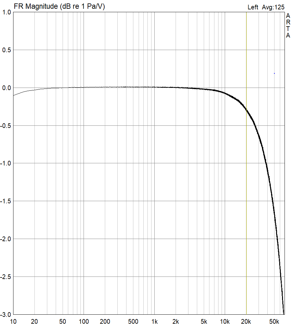
In the VCA frequency response graph, the dip at 10Hz is probably from the audio interface doing the measuring. The high roll-off was designed to give -0.3dB at around 20kHz, which seems to be what the graph is showing.
You can generate sweep tones in Audacity with Generate → Chirp.
The generalizations about measurements I give here come from a somewhat unscientific review of manufacturer’s websites for commonly well-regarded devices, along with the invaluable measurements of Amir Majidimehr and others at audiosciencereview.com.
NS10 frequency plots come from Phil Ward, “The Yamaha NS10 Story,” in Sound on Sound, 2008.
The boomy speaker plot is from a series of measurements in Philip Newell et al., “The Yamaha NS10M: Twenty Years a Reference Monitor. Why?” Reproduced Sound, 2001. While NS10s are a useful reference, the main reason I keep referencing them is that they’re what other people have researched—more self-perpetuating popularity, sorry.
I don’t get into it here, but frequency-dependent nonlinearities are often the result of using the wrong kind of capacitors in particular kinds of circuits. This does not mean that capacitors are always a significant source of distortion or that a particular kind of capacitor is “better” than another kind in every circuit. This is thoroughly explored in a series of articles on “Capacitor Sound” by Cyril Bateman, Electronics World 2002–2003.
For more info about the difficulties in measuring noise spectra, see Audio Precision, “FFT Scaling for Noise.” This is also the source of the graphic depicting a noise spectrum at two different resolutions.
Strictly speaking, you can actually define the noise density at a specific pitch with the Dirac delta equation. However, the noise density at that specific pitch will be infinity, not a useful measurement value.
Perceived noise levels aren’t quite the same as actual noise levels. See Csaba Horváth, Noise perception, detection threshold & dynamic range, 2023.
I’ve been unable to find any psychoacoustic studies on how the presence of noise affects the threshold of hearing. I am highly dubious about that—likely this is just because I am not sufficiently embedded in the field to know where to look.
An experiment with cochlear implant listeners found that in some cases added noise enhanced their ability to hear quieter sounds: Fan-Gand Zeng et al., “Human hearing enhanced by noise,” Brain Research 869, pp. 251–255, 2000.
Audacity, a free and open-source audio editor, has a built-in noise reduction algorithm. While other software is a little cagey about what it does, the algorithms are probably similar.
This translation of the Luigi Russalo quote was adapted from the original Italian. An English translation can be found in Luigi Russalo, trans. Barclay Brown, The Art of Noises, New York: Pendragon Press, 1986.
These somewhat idiosyncratic lists of movements and artists were influenced by Tara Rodgers insightful discussion about music history in Pink Noises: Women in Electronic Music and Sound, Durham, NC: Duke University Press, 2010. We need better histories of experimental music. Like with many histories, inclusivity happens somewhat automatically if we just cut out bad assumptions about Great Men being the creators of history and acknowledge the intersections that obviously exist across genres and movements (which are generally retrospectively defined by critics and historians). These lists I made are meant to be a step in this direction, though admittedly a small and inadequate step.
There’s a similar movement of thought where hyperobjectivity turns into hypersubjectivity in the Vienna circle of philosophers. They start out rejecting all kinds of philosophy in favor of physics, and end up saying that physics is only about comparing sentences. See especially the work of Rudolf Carnap and Otto Neurath.